how to use moving average crossover in binary options trading

Generating Trade Signals using Moving Average(MA) Crossover Strategy — A Python implementation

Moving averages are commonly used in technical analysis of stocks to predict the futurity toll trends. In this article, nosotros'll develop a Python script to generate purchase/sell signals using simple moving average(SMA) and exponential moving average(EMA) crossover strategy.

Photo by NICHOLAS CAPPELLO on Unsplash

— — — — — — — — — — — — — — — —
Disclaimer — The trading strategies and related information in this article is for the educational purpose only. All investments and trading in the stock market involve risk. Any decisions related to buying/selling of stocks or other financial instruments should but be made afterward a thorough research and seeking a professional assistance if required.
— — — — — — — — — — — — — — — —

Indicators such as Moving averages(MAs), Bollinger bands, Relative Strength Alphabetize(RSI) are mathematical technical analysis tools that traders and investors use to analyze the past and anticipate futurity cost trends and patterns. Where fundamentalists may runway economical data, almanac reports, or various other measures, quantitative traders and analysts rely on the charts and indicators to assistance interpret price moves.

The goal when using indicators is to identify trading opportunities. For example, a moving average crossover frequently signals an upcoming trend change. Applying the moving average crossover strategy to a price nautical chart allows traders to identify areas where the trend changes the management creating a potential trading opportunity.

Before we begin, yous may consider going through below article to go yourself accustomed with some common finance jargons associated with stock market.

What are Moving Averages ?

A moving boilerplate, likewise called equally rolling average or running boilerplate is a used to analyze the time-series data by computing a serial of averages of the different subsets of full dataset.

Moving averages are the averages of a serial of numeric values. They have a predefined length for the number of values to average and this prepare of values moves forrad as more data is added with time. Given a series of numbers and a fixed subset size, the first element of the moving averages is obtained past taking the average of the initial fixed subset of the number serial. And so to obtain subsequent moving averages the subset is 'shift forward' i.eastward. exclude the first chemical element of the previous subset and add the element immediately afterwards the previous subset to the new subset keeping the length fixed . Since it involves taking the average of the dataset over fourth dimension, it is as well called a moving hateful (MM) or rolling mean.

In the technical assay of fiscal data, moving averages(MAs) are among the virtually widely used trend following indicators that demonstrate the management of the market place's trend.

Types of Moving Averages

There are many different types of moving averages depending on how the averages are computed. In any time-series data analysis, the most commonly used types of moving averages are —

• Simple Moving Average(SMA)
• Weighted Moving Average(WMA)
• Exponential Moving Boilerplate (EMA or EWMA)

The just noteworthy difference between the various moving averages is the weight assigned to data points in the moving average period. Simple moving averages apply equal weight to all data points. Exponential and weighted averages utilize more weight to recent data points.

Among these, Simple Moving Averages(SMAs) and Exponential Moving Averages(EMAs) are arguably the virtually popular technical assay tool used past the analysts and traders. In this article, nosotros'll focus primarily on the strategies involving SMAs and EMAs.

Elementary Moving Average (SMA)

Simple Moving Boilerplate is one of the core technical indicators used by traders and investors for the technical analysis of a stock, index or securities. Simple moving boilerplate is calculated past adding the the endmost price of last n number of days and so diving by the number of days(time-period). Before we dive deep, let'southward first sympathize the math behind unproblematic averages.

We have studied how to compute average in schoolhouse and even in our daily life we often come beyond the notion of it. Permit's say you lot are watching a game of cricket and a batsman comes for batting. By looking at his previous v friction match scores— 60, 75, 55, eighty, l; you lot tin expect him to score roughly around threescore–70 runs in today's friction match.

By calculating the average of a batsman from his last 5 matches, yous were able to make a crude prediction that he'll score this much runs today. Although, this is a rough estimation and doesn't guarantee that he'll score exactly same runs, but still the chances are high. Also, SMA helps in predicting the hereafter tendency and make up one's mind whether an asset price will continue or reverse a bull or bear trend. The SMA is ordinarily used to identify tendency direction, just it can too exist used to generate potential trading signals.

Computing Simple moving averages — The formula for computing the SMA is straightforward:

The simple moving average = (sum of the an asset price over the past n periods) / (number of periods)

Source: Investopedia

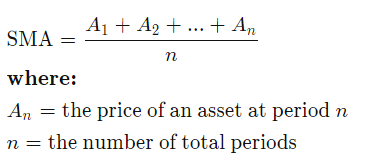
All elements in the SMA take the same weightage. If the moving average menstruum is five, then each element in the SMA will have a 20% (1/5) weightage in the SMA.

'n periods' can be anything. You can have a 200 day elementary moving average, a 100 hour simple moving boilerplate, a five 24-hour interval simple moving average, a 26 week unproblematic moving boilerplate, etc.

At present that we take accustomed ourselves with the basics, let'south leap to the Python implementation.

Calculating 20-day and l-solar day moving averages

For this example, I accept taken the 2 years of historical information of the Closing Price of UltraTech Cement Express stock(ULTRACEMCO as registered on NSE) from 1st Feb 2018 to 1st Feb 2020. You may choose your own set of stocks and the time flow for the analysis.

Permit's began past extracting the stock toll data from Yahoo Finance by using Pandas-datareader API.

Importing necessary libraries —

          import numpy as np            
import pandas equally pd
import matplotlib.pyplot as plt
import datetime
import                  

Extracting endmost price data of UltraTech Cement stock for the aforementioned fourth dimension-period —

          # import package
import pandas_datareader.data as web          # set up commencement and end dates            
commencement = datetime.datetime(2018, ii, 1)            
terminate = datetime.datetime(2020, 2, 1)                    # extract the closing price data
ultratech_df = web.DataReader(['ULTRACEMCO.NS'], 'yahoo', kickoff = outset, cease = end)['Close']
ultratech_df.columns = {'Close Price'}
ultratech_df.head(ten)        

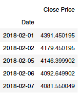
Annotation that SMAs are calculated on closing prices and non adapted close because we desire the trade signal to be generated on the price data and not influenced past dividends paid.

Observe full general price variation of the endmost price for the requite menstruation —

          ultratech_df['Close Toll'].plot(figsize = (15, 8))
plt.grid()
plt.ylabel("Price in Rupees"
plt.show()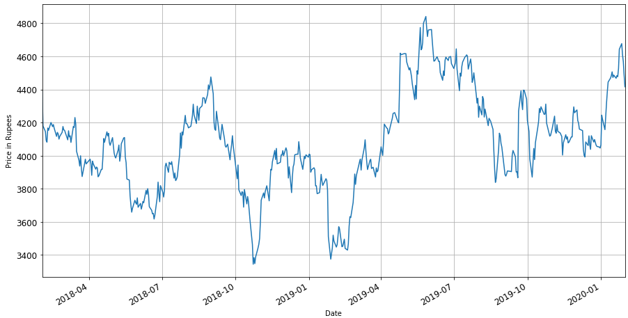        

Create new columns in our dataframe for both the long(i.e. 50 days) and short (i.eastward 20 days) elementary moving averages (SMAs) —

          # create xx days simple moving average cavalcade
ultratech_df['20_SMA'] = ultratech_df['Close Cost'].rolling(window = xx, min_periods = one).mean()          # create fifty days simple moving average column
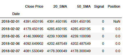
ultratech_df['50_SMA'] = ultratech_df['Close Price'].rolling(window = fifty, min_periods = 1).mean()          # display get-go few rows
ultratech_df.caput()        

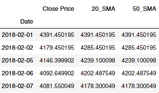
In Pandas, dataframe.rolling() function provides the feature of rolling window calculations. min_periods parameter specifies the minimum number of observations in window required to have a value (otherwise outcome is NA).

Now that we have 20-days and l-days SMAs, side by side we see how to strategize this information to generate the trade signals.

Moving Average Crossover Strategy

At that place are several ways in which stock market place analysts and investors tin use moving averages to analyse cost trends and predict upcoming modify of trends. At that place are vast varieties of the moving boilerplate strategies that can be adult using different types of moving averages. In this article, I've tried to demonstrate well-known simplistic yet constructive momentum strategies — Simple Moving Average Crossover strategy and Exponential Moving Average Crossover strategy.

In the statistics of time-serial, and in particular the Stock market technical analysis, a moving-average crossover occurs when on plotting, the two moving averages each based on unlike time-periods tend to cross. This indicator uses two (or more) moving averages — a faster moving average(short-term) and a slower(long-term) moving average. The faster moving average may be 5-, 10- or 25-mean solar day period while the slower moving average can be 50-, 100- or 200-24-hour interval period. A short term moving boilerplate is faster because it but considers prices over short catamenia of fourth dimension and is thus more reactive to daily price changes. On the other hand, a long-term moving average is accounted slower every bit information technology encapsulates prices over a longer period and is more than lethargic.

Generating Trade signals from crossovers

A moving average, as a line by itself, is often overlaid in toll charts to betoken price trends. A crossover occurs when a faster moving average (i.due east. a shorter period moving boilerplate) crosses a slower moving average (i.e. a longer period moving average). In stock trading, this meeting point can be used equally a potential indicator to buy or sell an nugget.

• When the short term moving average crosses in a higher place the long term moving boilerplate, this indicates a purchase signal.
• Contrary, when the short term moving average crosses below the long term moving average, it may be a good moment to sell.

Having equipped with the necessary theory, at present let's continue our Python implementation wherein we'll try to incorporate this strategy.

In our existing pandas dataframe, create a new column 'Betoken' such that if xx-twenty-four hour period SMA is greater than l-day SMA then set Signal value as 1 else when fifty-day SMA is greater than 20-day SMA then set it'south value as 0.

          ultratech_df['Point'] = 0.0
ultratech_df['Indicate'] = np.where(ultratech_df['20_SMA'] > ultratech_df['50_SMA'], ane.0, 0.0)        

From these 'Signal' values, the position orders can exist generated to represent trading signals. Crossover happens when the faster moving average and the slower moving average cross, or in other words the 'Signal' changes from 0 to 1 (or 1 to 0). And so, to incorporate this information, create a new cavalcade 'Position' which zippo simply a day-to-day departure of the 'Betoken' cavalcade.

          ultratech_df['Position'] = ultratech_df['Bespeak'].unequal()          # display first few rows
ultratech_df.caput()        

• When 'Position' = 1, it implies that the Signal has changed from 0 to 1 meaning a short-term(faster) moving average has crossed in a higher place the long-term(slower) moving average, thereby triggering a buy call.
• When 'Position' = -ane, information technology implies that the Betoken has inverse from one to 0 pregnant a brusque-term(faster) moving average has crossed below the long-term(slower) moving average, thereby triggering a sell phone call.

At present let's visualize this using a plot to make information technology more than articulate.

          plt.figure(figsize = (twenty,10))
# plot shut price, curt-term and long-term moving averages            
ultratech_df['Close Price'].plot(color = 'k', label= 'Close Price')            
ultratech_df['20_SMA'].plot(colour = 'b',label = 'xx-solar day SMA')            
ultratech_df['50_SMA'].plot(color = 'g', label = 'fifty-twenty-four hours SMA')          # plot 'buy' signals
plt.plot(ultratech_df[ultratech_df['Position'] == 1].index,            
            ultratech_df['20_SMA'][ultratech_df['Position'] == ane],            
            '^', markersize = xv, color = 'g', characterization = 'buy')          # plot 'sell' signals
plt.plot(ultratech_df[ultratech_df['Position'] == -i].index,            
            ultratech_df['20_SMA'][ultratech_df['Position'] == -ane],            
            '5', markersize = 15, color = 'r', characterization = 'sell')
plt.ylabel('Toll in Rupees', fontsize = 15 )
plt.xlabel('Engagement', fontsize = 15 )
plt.title('ULTRACEMCO', fontsize = 20)
plt.fable()
plt.grid()
plt.show()        

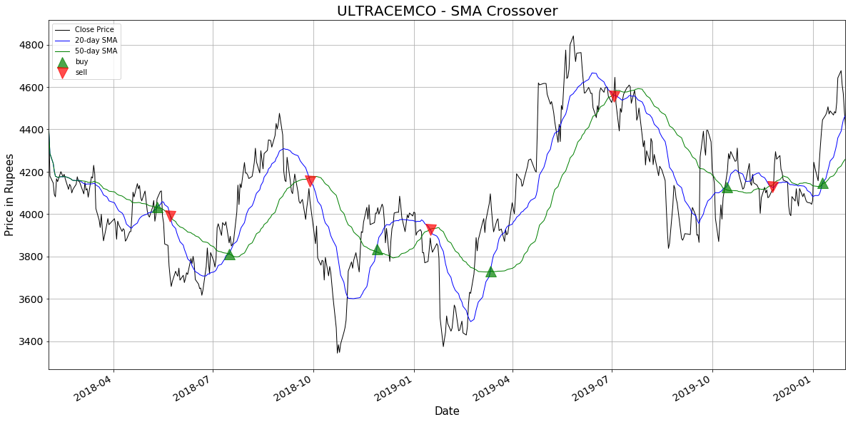
As you tin run into in the above plot, the blue line represents the faster moving boilerplate(20 day SMA), the green line represents the slower moving average(50 day SMA) and the black line represents the actual closing price. If yous carefully observe, these moving averages are cypher but the smoothed versions of the actual cost, but lagging by certain menstruation of fourth dimension. The brusque-term moving average closely resembles the bodily toll which perfectly makes sense as it takes into consideration more recent prices. In dissimilarity, the long-term moving average has comparatively more lag and loosely resembles the actual price curve.

A indicate to buy (as represented by green upwards-triangle) is triggered when the fast moving average crosses above the slow moving average. This shows a shift in trend i.e. the boilerplate cost over final 20 days has risen in a higher place the average price of past 50 days. Too, a indicate to sell(as represented by red downwards-triangle) is triggered when the fast moving boilerplate crosses below the slow moving average indicating that the average price in last 20 days has fallen below the average cost of the final l days.

Exponential Moving Average (EMA or EWMA)

And so far we have discussed the moving boilerplate crossover strategy using the elementary moving averages(SMAs). It is straightforward to observe that SMA fourth dimension-serial are much less noisy than the original price. Nevertheless, this comes at a price — SMA lag the original toll, which means that changes in the trend are only seen with a delay of L days. How much is this lag Fifty? For a SMA moving average calculated using M days, the lag is roughly around Yard/2 days. Thus, if we are using a l days SMA, this means we may exist late by almost 25 days, which can significantly affect our strategy.

One style to reduce the lag induced by the employ of the SMA is to utilise Exponential Moving Average(EMA). Exponential moving averages give more than weight to the most recent periods. This makes them more reliable than SMAs as they are insufficiently better representation of the recent operation of the asset. The EMA is calculated every bit:

EMA [today] = (α x Toll [today] ) + ((1 — α) x EMA [yesterday] )

Where:
α = 2/(N + one)
North = the length of the window (moving average period)
EMA [today] = the electric current EMA value
Price [today] = the current endmost price
EMA [yesterday] = the previous EMA value

Although the calculation for an EMA looks bit daunting, in practice it's elementary. In fact, it's easier to calculate than SMA, and besides, the Pandas ewm functionality will do it for you in a single-line of code!

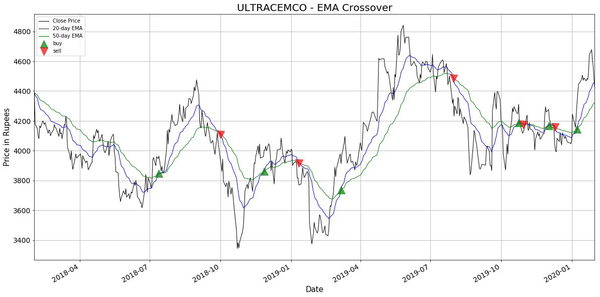
Having understood the basics, let'south attempt to incorporate EMAs in place of SMAs in our moving average strategy. We're going to use the aforementioned code as higher up, with some minor changes.

          # set start and end dates
start = datetime.datetime(2018, two, ane)
stop = datetime.datetime(2020, 2, 1)          # extract the daily closing toll data
ultratech_df = web.DataReader(['ULTRACEMCO.NS'], 'yahoo', first = kickoff, end = terminate)['Shut']
ultratech_df.columns = {'Close Price'}          # Create 20 days exponential moving average column
ultratech_df['20_EMA'] = ultratech_df['Shut Price'].ewm(span = xx, adjust = Imitation).mean()          # Create 50 days exponential moving average column
ultratech_df['50_EMA'] = ultratech_df['Close Toll'].ewm(bridge = fifty, accommodate = False).mean()          # create a new column 'Signal' such that if twenty-24-hour interval EMA is greater   # than 50-day EMA then ready Signal as 1 else 0
              ultratech_df['Signal'] = 0.0              
ultratech_df['Point'] = np.where(ultratech_df['20_EMA'] > ultratech_df['50_EMA'], 1.0, 0.0)
                    # create a new column 'Position' which is a solar day-to-day departure of # the 'Signal' column
ultratech_df['Position'] = ultratech_df['Signal'].diff()          plt.figure(figsize = (20,ten))
# plot close toll, curt-term and long-term moving averages            
ultratech_df['Close Price'].plot(colour = 'k', lw = 1, label = 'Close Price')            
ultratech_df['20_EMA'].plot(color = 'b', lw = one, characterization = '20-mean solar day EMA')            
ultratech_df['50_EMA'].plot(color = 'chiliad', lw = 1, characterization = '50-mean solar day EMA')          # plot 'buy' and 'sell' signals
plt.plot(ultratech_df[ultratech_df['Position'] == 1].index,            
            ultratech_df['20_EMA'][ultratech_df['Position'] == i],            
            '^', markersize = 15, colour = 'g', characterization = 'purchase')          plt.plot(ultratech_df[ultratech_df['Position'] == -1].index,            
            ultratech_df['20_EMA'][ultratech_df['Position'] == -1],            
            'v', markersize = xv, color = 'r', characterization = 'sell')          plt.ylabel('Price in Rupees', fontsize = 15 )
plt.xlabel('Date', fontsize = 15 )
plt.championship('ULTRACEMCO - EMA Crossover', fontsize = 20)
plt.fable()
plt.grid()
plt.show()        

The following extract from John J. White potato's work, "Technical Analysis of the Financial Markets" published past the New York Establish of Finance, explains the advantage of the exponentially weighted moving average over the simple moving average—

"The exponentially smoothed moving average addresses both of the bug associated with the simple moving average. First, the exponentially smoothed average assigns a greater weight to the more than recent data. Therefore, it is a weighted moving boilerplate. But while it assigns lesser importance to by toll information, it does include in its calculation all the information in the life of the instrument. In add-on, the user is able to adjust the weighting to give greater or lesser weight to the almost contempo day's price, which is added to a percentage of the previous day's value. The sum of both percentage values adds upward to 100."

Complete Python Program

The office 'MovingAverageCrossStrategy()' takes following inputs —

• stock_symbol —(str) stock ticker as on Yahoo finance.
  Eg: 'ULTRACEMCO.NS'
• start_date — (str)start analysis from this date (format: 'YYYY-MM-DD')
  Eg: '2018-01-01'.
• end_date— (str)finish analysis on this date (format: 'YYYY-MM-DD')
  Eg: '2020-01-01'.
• short_window— (int)look-back period for short-term moving average.
  Eg: five, ten, 20
• long_window — (int)look-back catamenia for long-term moving boilerplate.
  Eg: 50, 100, 200
• moving_avg— (str)the type of moving average to employ ('SMA' or 'EMA').
• display_table — (bool)whether to display the date and toll table at buy/sell positions(True/False).

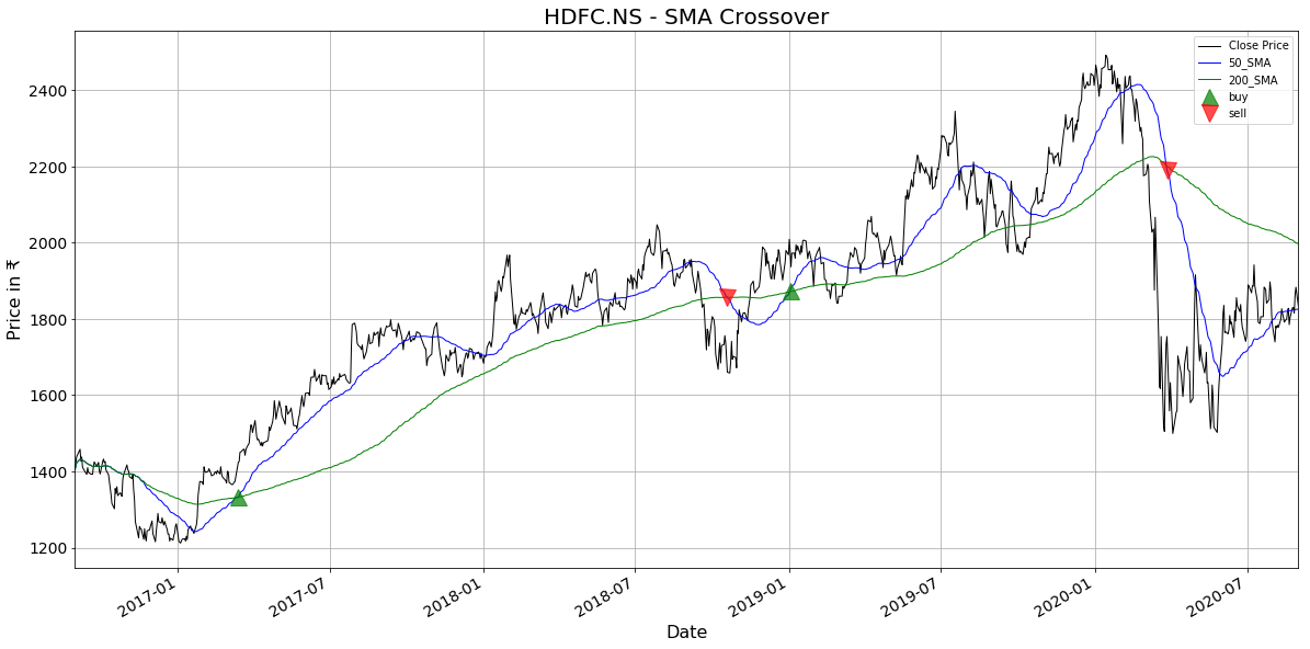
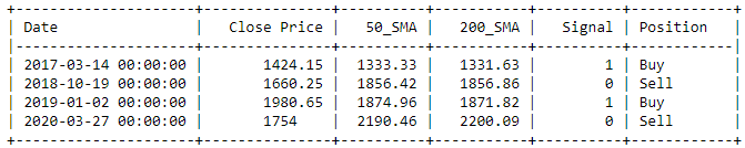
Now, let's exam our script on terminal 4 years of HDFC depository financial institution stock. We'll be using 50-twenty-four hours and 200-mean solar day SMA crossover strategy.

Input:

          MovingAverageCrossStrategy('HDFC.NS', '2016-08-31', '2020-08-31', l, 200, 'SMA', display_table = True)        

Output:

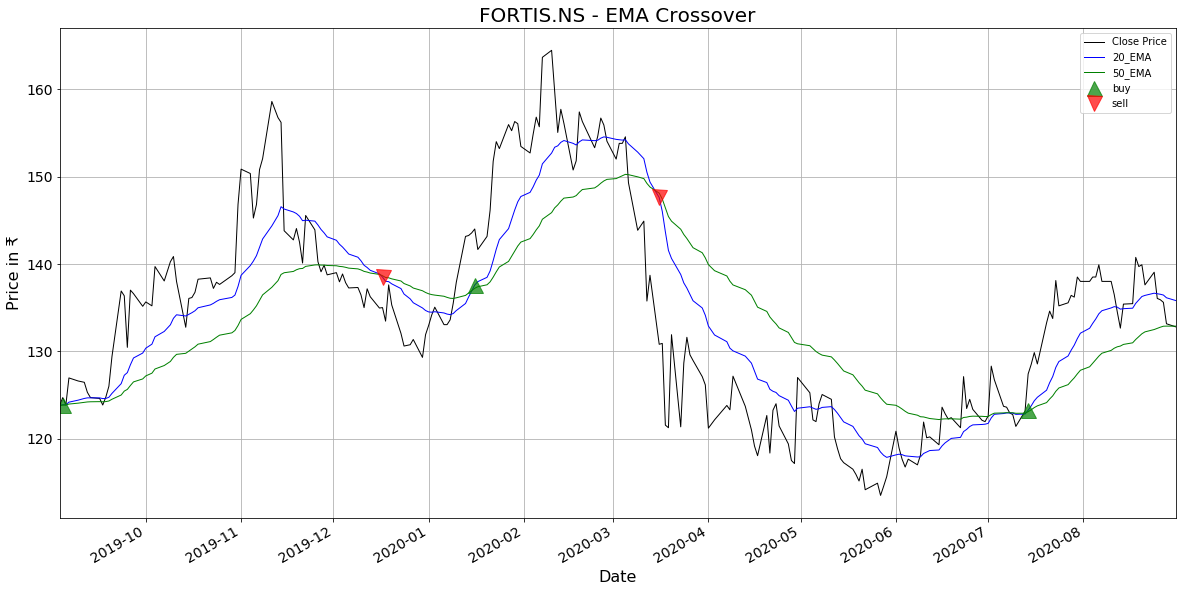
How about Fortis Healtcare stock? This time we analyze past 1 year of data and consider 20-days and 50-days EMA Crossover. Also, this time we won't be displaying the tabular array.

Input:

          MovingAverageCrossStrategy('FORTIS.NS', '2019-08-31', '2020-08-31', 20, 50, 'EMA', display_table = False)        

Output:

Due to the central difference in the manner they are calculated, EMA reacts apace to the price changes while SMA is comparatively slow to react. But, one is non necessarily ameliorate than another. Each trader must decide which MA is meliorate for his or her particular strategy. In full general, shorter-term traders tend to use EMAs because they desire to be alerted as presently every bit the price is moving the other way. On the other hand, longer-term traders tend to rely on SMAs since these investors aren't rushing to human action and prefer to be less actively engaged in their trades.

Beware! As a tendency-following indicators, moving averages work in markets that have clear, long term trends. They don't work that well in markets that can be very choppy for long periods of time. Moral of the story — moving averages are not a one-size-fits-all holy grail. In fact, in that location is no perfect indicator or a strategy that volition guarantee success on each investment in all circumstances. Quantitative traders often utilise a diversity of technical indicators and their combinations to come up with different strategies. In my subsequent manufactures, I will try to innovate some of these technical indicators.

End notes

In this article, I showed how to build a powerful tool to perform technical analysis and generate trade signals using moving average crossover strategy. This script can be used for investigating other company stocks by simply changing the argument to the function MovingAverageCrossStrategy().

This is merely the commencement, information technology is possible to create much more sophisticated strategies which I'll be looking forward to.

Looking Forward

• Incorporate more than strategies based on indicators similar Bollinger bands, Moving Average Convergence Divergence (MACD), Relative Strength Index(RSI) etc.
• Perform backtesting to evaluate the performance of different strategies using advisable metrics.

Source: https://towardsdatascience.com/making-a-trade-call-using-simple-moving-average-sma-crossover-strategy-python-implementation-29963326da7a

Posted by: jenkinswasuff.blogspot.com

Share this post